Crib notes on implementing machine learning using neural networks in C
This document is a work in progress, not all sections are filled in yet and the editing of the pieces that are filled in is not complete yet. The structure is rather ad-hoc as well still, I’m not sure how much introduction/education I need to do versus going straight into implementation details. Or in other words: Feedback welcome.
After the introduction, there’s a tutorial on building a neural network using genetic algorithms, and after the tutorial I’m describing more detailed things I encountered while implementing neural networks.
As a hobby I've been playing with implementing machine learning algorithms
in my spare time, and specifically a neural network to analyze images to
recognize numbers inside an image.
There are many many books about the fundamentals and theory of various
aspects of machine learning, and I have enjoyed reading quite a few of
these. I'm an engineer more than a scientist, so I want to play with how you
build machine learning systems, how you make them tick and what you can do
to make them do cool things.
In this blog/article I'm writing down some of the things I learned about
implementing neural networks, what worked, what didn't work and why. Initially it’ll read like a set of rambling paragraphs; I’ll be editing and adding content for quite some time to go.
Many of the books cover the theory but skip over the details of how to actually
build a working system. I know many (free) implementations exist, and very
likely I made many mistakes that people will point out (and I'll learn from
that and update this article)... but for me the fun is in the building, and
I hope what I write here is useful for others who also enjoy building
software.
My curiosity was peaked by a mainstream press article about a research team using a very large number of servers to build a neural network to separate/classify pictures of dogs and cats. I started to wonder if this wouldn’t be a task the computers in my basement should be able to do; what is so hard that makes you need such a huge farm. I also immediately realized I was in way over my head and that I should start with something simpler. A few Google queries later, and I decided to start with the simple task of recognizing numbers in a fixed sized image (see http://www.nithinrajs.in/ocr-using-artificial-neural-network-opencv-part-2-preprocessing/).
.....XX........X .....XXXXXXXXXXX ....XX.......... ....X........... ...XX........... ..XXXXXXXX...... ..XXXXXXXXXXX... ..........XXXXX. ............XXXX .............XXX ..............XX ..............XX ..............XX .X...........XX. .XX.........XX.. .XXXXX...XX..... | ........XXX..... ....XXXXXXXXXX.. ...XXXX....XXXX. ..XXX........XXX .XXX..........X. .XX............. .XX....XXXXX.... XXX.XXXXXXXXXX.. XXXXXX......XXXX XXXX..........XX XXXX..........XX .XXX..........XX .XXX..........XX ..XX.........XXX ..XXXX......XXX. ....XXXXXXXXXX.. | XXXXXXXXXXXXXXXX XXXXXXXXXXXXXXXX XXXXXXXXXXXXXXXX ...........XXXX. ..........XXXX.. .........XXXX... ........XXXX.... ........XXXX.... .......XXXX..... ......XXXX...... .....XXXXX...... .....XXXX....... .....XXXX....... ....XXXXX....... ....XXXX........ ....XXXX........ |
The rest of this article is about the various engineering decisions and experiments I did while working on this much simpler problem. If I ever get my basement computers to recognize cats and dogs, be assured that I will write about that somewhere as well.
It turns out that neural networks are very resilient against a common set of programming errors; I found many times that the neural network would still train (but slowly) and work reasonably despite an obvious bug in the code. If you have a network that trains slowly or trains but then saturates in result prematurely, consider a severe programming bug as one of the possible reasons.
This will be a step-by-step, build your own neural network tutorial showing source code snippets for each step. Full source for each section is available at the link mentioned at the end of each section.
A note of warning: In several places I deviate from the more conventional approaches; if you want to use this material as preparation for say a class or an exam, you are more than welcome to do so but expect to be challenged by the teacher on some of the approaches. Detailed discussion these decisions is in the pages after the primer.
In this tutorial I’m going to be using the training set from http://www.nithinrajs.in/ocr-using-artificial-neural-network-opencv-part-2-preprocessing
since it’s well prepared and convenient to parse in a small amount of code; this tutorial is about neural networks, not about parsing data sets into memory after all.
The basic data structure to keep track for a training item will be struct input:
#define INPUTS 257
#define MAXINPUT 8192
struct input {
double values[INPUTS];
int output;
};
and for convenience, we just make a static array for all the inputs:
struct input inputs[MAXINPUT];
To make a long story short, the example code for step 1 of this tutorial can be found at http://ai.fenrus.org/section1.
What’s a neural network without neurons?
Lets start with a very simple neuron:
#define NSIZE 32
struct neuron {
double value;
int inputs[NSIZE];
double weights[NSIZE];
};
Our neurons have 32 bit synapses coming into them, and each synapses has an origin neuron (input) and a weight.
Neurons don’t just have links, they have an activation function.
For this tutorial we’re using a pretty simple activation function:
This function is very fast to compute using a simple C function:
static double activation(double sum)
{
double r;
r = 0.05 * sum + 0.1;
if (sum > 0)
r += 0.8;
return r;
}
If you’ve been reading other articles about neural networks, you’d have read things about sigmoid functions using exponents or hyperbolic tangents. Mathematicians love such functions, however computers don’t, those mathematical functions are quite expensive to compute. The simple activation function above computes much faster (easily 10x faster) than a sigmoid function, and my experiments show (see the details later on) that the quality and training rate of a network with the simple function are the same as networks that use the expensive functions.
A single neuron is rather boring.. you can’t even calculate its value. So lets turn a bunch of these into a network:
#define NETSIZE 768
struct network {
struct neuron neurons[NETSIZE];
int correct;
double score;
};
With this, now we can finally actually calculate the value of a neuron. This is simple, add up value of the neurons connected via the input synapses, multiplied by their respective weights.
We’re going to treat synapse number zero, and hardwire it to the bias neuron.
So the summing will look like this in the do_neuron() function:
sum = network->neurons[index].weights[0]; /* The bias */
for (i = 1; i < NSIZE; i++) {
int from = network->neurons[index].inputs[i];
sum += network->neurons[index].weights[i] *
network->neurons[from].value;
}
The second part of the neuron evaluation is to see the neuron has changed value; we’re going to need to iteratively calculate the neuron values in the network and stop the calculation once no neurons are changing their value anymore.
So to calculate the entire network one time, the code is still quite simple:
static int do_network_once(struct network *network)
{
int change_count = 0;
int i;
for (i = INPUTS + 1; i < NETSIZE; i++)
change_count += do_neuron(network, i);
return change_count;
}
In the next section we’ll add input and output to the network, so that we can calculate the output of the network given a specific input.. but for now, you can look at the code that we have so far at http://ai.fenrus.org/section3
By convention, input neurons (that represent the input data) are at the start of the network, while output neurons are at the end of the network.
.
There seems to be a fundamental split in the approach to training a neural network between Back Propagation and Genetic Algorithms.
The idea behind back propagation is a very simple one: Consider the neural net as one big mathematical function, with the weights of the various synapsis as inputs to that function, and some measure of error as the output of the function. To minimize the error (e.g. training), one takes the partial derivative of these inputs (the weights) and then you pick one of the various tools from basic numerical methods to find the value for each weight that leads to a (local) minimum in the final error value.
To make this practical, a few approximations are made in the math behind this, and the adjusting of the weights happens in parallel rather than one-by-one, but neither of these change the fundamental idea (the combination of the various approximations and the specific numerical methods used define the exact algorithm and some of them have fancy names like RPROP-)
For back propagation to be possible, there are quite a few limits on the structure of the neural network as well as on the activation function of the neuron; most of the entry level literature only describes a strict feed-forward architecture with one hidden layer. While many successes have been had with neural networks using back propagation, I’m dubious about its scaling to larger network structures with multiple layers; the individual partial derivatives end up shrinking for each extra layer reducing the efficiency of training beyond the first hidden layer to the point where I don’t like the odds of getting it to work well. Wikipedia calls this the vanishing-gradient problem.
I’ll be honest, in college I detested partial derivatives. Not because they are hard (they are not), but because they tend to be tedious. So for this experiment, I started out as partial against back propagation and picked the other solution: Genetic Algorithms. Even with this in mind, I realize that back propagation is very good at small optimizations in the network, and I may end up with a combination of Genetic Algorithms and a variant of back propagation.
In the world of GA one describes a problem as a “chromosome”, and you create a set of distinct networks that are different. The best of these networks get to combine, where a new network is a combination of the old network and the new network, with an occasional random mutation thrown in. You end up with a evolution-inspired directed random search that has shown to be able to optimize quite a variety of problems. At work I’ve experimented with GA’s for several problems for example.
Unlike back propagation, GAs don’t prescribe any specific network structure as long as the network can be expressed in a “chromosome”.
I decided early on that I wouldn’t just optimize (e.g. evolve) the weights of the neural network, but the actual structure of the network as well (e.g. which neurons connect to which neurons).
In the implementation, I chose to give each neuron a fixed (maximum) number of incoming synapses with corresponding weights:
#define NSIZE 32
struct neuron {
double value;
double sum;
int inputs[NSIZE];
double weights[NSIZE];
};
I’ve not put any restrictions on the origin of these links. Explicitly this allows for cycles in the network as well as “self linking” of neurons. I don’t know apriori if those are useful or not, but I figure that if they are useful, the GA will end up going there; I see no reason to ban these kind of constructs.
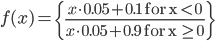
The activation function is what makes the neural network its non-linear nature; the biological equivalent is basically a step function but for various reasons, a sigmoid shape is always used for computer equivalents. The most popular forms of activation functions are the exponent based sigmoid (http://en.wikipedia.org/wiki/Sigmoid_function) for inputs that map best in a range from [0, 1] and a tanh() based function for inputs that map best to a range [-1, 1].
For the problem at hand I picked the basic function. Note that when you implement a neural network, you’ll find quickly that you end up spending a LOT of cpu time in just this function, easily over 50% of the total cpu cycles.
(the sigmoid function from the wikipedia URL above)
It’s natural to try to optimize the compute time of this function, but there are some caveats:
For learning to work well, the function needs to be strictly monotonous, e.g. a higher input value must lead to a higher output value,
 for any positive
  and
and 
I’ve tried to violate this rule to cut down computation time, but the result is that the network doesn’t train much at all. It comes down to the fact that minimization algorithms (BP or GA or, well, any) are not good at coping with plateaus and work much better if there is some gradient in the right direction, even if the gradient is small.
The second constraint is that if you want to use back propagation, the activation function needs to be differentiable, and ideally continuously differentiable.
Since I’m not using BP (yet), I’m going to experiment with a simpler-to-compute activation function like the one below:
This function is much faster to compute than the exponent based sigmoid. Measurements show that this function works at least as good as a sigmoid function:
In this graph, the red line is the simple, linear-with-a-jump function and the blue line is the exponent based sigmoid function. The simple linear-with-a-jump function slightly outperforms the traditional function in terms of learning rate.
There are 10 numbers (digits) in the problem, and I’ve defined the network to have 10 outputs, one for each possible digit. The “winner”, e.g. recognized digit, is the output with the highest value, no matter how low or high in absolute terms.
This is simple and works well for problems that have a small number of discrete possible outputs (“dog” vs “cat”, digits etc).
To use a GA, you need each network to have a “score” that you want to optimize. I personally like numbers that go up, e.g. higher is better, but it’s equally valid to use some sort of error metric where you then try to minimize the error. When designing the score function, the key thing to remember is “you get what you reward”.
It’s tempting to use a simple, discrete metric as the score; in this case, the number of correctly identified images. However, this is not a good idea and won’t work well in practice. For learning to work, it’s important that the score function rewards even the smallest improvement in the network by at least a little bit, so that the direction of learning is clear and so that small improvements can be selected, and small steps backwards can be eliminated/ignored.
The score function I’ve picked gives 10 points for each correctly identified digit and 0 points for each incorrectly identified digit. But in addition to that, for a correctly identified digit, the score is increased by the difference in output from the winning output neuron and the second-highest output neuron, which is a fraction between 0.0 and 1.0
Also, for incorrectly identified digits, the score is subtracted by the difference in output of the selected output neuron and the output neuron that should have been selected, which is in the range of -1.0 to 0.0.
These two tweaks together reward, in small fractions of the score, either more clear winners, or less wrong losers. In various other parts of this blog posting I’ll describe other things I’ve included in the score to reward or punish specific behaviors.
In a strict feed-forward network, evaluating the output values of the network is as simple as doing a single pass, from left to right over each of the neurons. However, in a free-form network, it’s a little more complex. For gigantic networks you can consider doing some form of asynchronous, multi-threaded evaluation. But for medium sized networks, just calculating the whole network several times until a steady-state is achieved is a relatively easy-to-implement solution. Since loops are possible, you need to build in a cut off, and since each round of evaluation takes cpu time, it’s advisable to reduce the network score a little each iteration of calculation to reward easier to evaluate networks.
I first tried implement the neuron bias with an explicit bias value for each neuron, including dealing with it in the GA mutation/etc. For Back Propagation, it’s really painful to do this, and it’s much easier to just insert a Bias Neuron which always has the value of 1, and then make sure that each neuron has a link to this bias neuron.
After having worked with the neural network program for a bit, it became clear that adding more synapses per neuron actually degraded the performance of the network. In a way, this is not surprising, More-than-needed synapses effectively add noise to the system, and too much noise obviously makes learning a lot harder. However, it’s not as simple as globally reducing the number of synapses (NSIZE), the need for the number of synapses is not uniform throughout the network.
The solution I implemented was both simple and effective: In addition to the normal mutate (tune) phase of the GA engine, I added a separate pass to try to delete (read: set the weight to zero) synapses as a mutation phase. As an additional step, I count the number of active (e.g. reachable when backtracking from the output neurons) neurons and synapses in the network. Each active neuron and synapse gets a small amount subtracted from the total score, so that there is a reward for removing “dead” synapses and neurons. In the various experiments, this pruning stage ends up rather effective in improving the learning rate, although care had to be taken to avoid pruning aggressively before the network has done some basic learnings. There is a pathological case where too early pruning cuts away many of the basic links that the network needs to do early phases of learning.
Specifically, I avoid pruning until the network reaches a 50% success rate to avoid these pathological cases.
The network has to start somewhere, both in terms of structure and in terms of weights.
The next section discusses how to initialize the weights of the synapses, but before going there, the initial network structure impacts learning speeds quite a lot.
I’ve settled on a configuration where each neuron has a fixed number of synapses (typically 8) come from an input neuron, while all other synapses are just randomly initialized. Without this “use an input” special case, the network will take a lot of time just learning where the input neurons are, and this is a waste of time.
The most common advice in the various articles and books is to initialize your neural network with random values for the weights, and for a back-propagation network you pretty much need to. In a previous section I wrote about the advantages that pruning the network yields, and this made me wonder how much better a random initialized network is compared to an all-zeros (e.g. fully pruned to nothing) network at the start, where the network grows up instead.
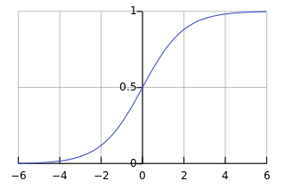
I’ve tried both methods (see the graph below) and it turns out that an all-zeros network starts out learning a lot (2x) faster than a random-populated network, but the all-zeros networks sometimes hit a ceiling where their learning rate slows down significantly, while the random-populated networks generally keep learning slower-but-steady and overtaking these few all-zeros networks. As a side bonus, the networks coming out of the all-zeros part are simpler and evaluate roughly 2x faster than the random-populated networks.
There is an opportunity here to find a hybrid approach that has the initial learning rate of the all-zeros network but the staying-power of the random-populated network. With the GA-island-approach in these tests, I plan to experiment with a setup where some islands are all-zeros and other networks are random-populated.
In this graph, the red dots, and the red fitted line, are from a set of all-zeroes runs, while the blue dots and blue fitted line are from random-populated networks, Both are done using 300 images from the training set for digit recognition and the Y-axis denotes the percentage of correct recognitions on the training set.
The training set from the problem at hand has 3050 entries. The CPU time needed to evaluate a network is linearly proportional to the number of training entries. One thing that is obvious is that while cpu time is linear with the number of entries, the training value is not: Going from 100 to 101 entries adds more new learning than going from 3000 to 3001 entries.
This provides an obvious opportunity to optimize:
Start with a small-but-relevant training set, and only increase this training set has reached a high enough (90% success) success rate that it’s worth adding more samples to the training set.
In the island setup I use for the GA engine, each island gets its own training subset to reduce the impact of monocultures. In addition, rather than pure adding more samples to the training set at reaching the success bar, the island that reaches the 90% bar also gets to see a whole new area of the training set, not just additional samples.
As I described in the pruning section, having too many synapses per neuron creates noise issues that prohibit learning fast.. yet too few synapses reduces the total capacity to learn. One of the tricks that worked well is to have a dynamic limit to the number of synapses, and to increase this limit each time the training set grows. Effectively, first the network learns, with a small number of synapses from a small training set, and each time it gets to learn more, it also gets a higher synapses budget allocated.
A rate of 1 extra synapse per 100 training samples worked quite well.
Initially I had implemented crossover by deciding, at random, for each neuron individually which of the two parents to pick from. The results were certainly not great for this approach, and I quickly switched to randomly picking the crossover point; neurons on one side of this point come from parent 1, while the neurons after this point come from parent 2. In hindsight, this is obvious; the crossover-point strategy allows complete structures to be inherited between parents.
to be written
The theory behind Genetic Algorithms is elegant in its simplicity, but when building an actual GA system, there are some practical considerations. The foremost problem with Genetic Algorithm Systems is that GA’s have a tendency to get a monoculture in the population where an early dominant neural net will effectively take over and causes the system to lose all its diversity. It’s diversity that allows new structures to be created; once a monoculture with a dominant neural net gets established, learning rates tend to slow to a crawl.
There’s four things I’ve done to limit the damage from monocultures: creatings islands, eradicating close duplicates, aging and split training sets.
Using isolated “islands” is a common technique to limit the damage from monocultures. You just make, say, 4 independent pools of networks. Inside each of these pools you let the GA do its thing but you keep the pools separated. If one of these pools hits a monoculture, there are still three others that make faster progress. I’ve gotten the best results with islands when I let each island send (a copy of) its best network to the main island on a regular basis; this creates genetic diversity in the main island with several strong, but independently evolved systems.
Removing near duplicate networks is also an easy way to reduce the occurrence of monocultures. Detecting pure duplicates is trivial, but not sufficient. I’ve taken the easy approach: during the sorting phase of the population, if two networks have a score that is very close (say within a score of 0.1) I immediately remove the worst of the two from the population. This enforces there to be differences between the individual networks, and while not perfect, tends to help reduce the chance of getting a monoculture with a dominant structure.
The third option is to introduce aging; sometimes implementers remove specimens older than a certain number of iterations, but that runs the risk of completely removing a good solution. I’ve done experiments where I let the age of the network count in the score of the network, but not with great success and I don’t have this in my current codebase.
The final method I used was to give each island a separate part of the training set to train on; this increases variety between the islands and helps the master island to stay diverse.
to be written
(one thread per island versus one thread per individual as part of generation jumps. for large networks, asynchronous network evaluation?)
http://www.ai-junkie.com/ann/evolved/nnt1.html
http://www.nithinrajs.in/ocr-using-artificial-neural-network-opencv-part-2-preprocessing/
http://msdn.microsoft.com/en-us/magazine/jj658979.aspx
Arjan van de Ven works for Intel Corporation as a Senior Principal Engineer building Android operating systems. His job has nothing to do with machine learning or neural networks, and the work in this blog posting has nothing to do with Intel Corporation.
To give feedback, ask questions or otherwise complain about this blog posting, please send your comments to arjanvandeven@gmail.com